
I recently participated in the Kaggle-hosted data science competition How Much Did It Rain II where the goal was to predict a set of hourly rainfall levels from sequences of weather radar measurements. I came in first! I describe my approach in this blog post.

My research lab supervisor Dr John Pinney and I were in the midst of developing a set of deep learning tools for our current research programme when this competition came along. Due to some overlaps in the statistical tools and data sets (neural networks and variable-length sequences, in particular) I saw it as a good opportunity to validate some of our ideas in a different context (at least that is my post hoc justification for the time spent on this competition!). In the near future I will post about the research project and how it relates to this problem.
One of things which inspired me to write this up, other than doing well in the competition, was the awesome blog post by Sander Dieleman where he describes his team’s winning approach in another Kaggle competition I took part in. So following the outline of that article, here’s my solution to this problem.
Introduction
The problem
The goal of the competition was to use sequences of polarmetric weather radar data to predict a set of hourly rain gauge measurements recorded over several months in 2014 over the US midwestern corn-growing states. These radar readings represent instantaneous precipitation rates and is used to estimate rainfall levels over a wider area (e.g. nationwide) than can practically be covered by rain gauges.
For the contest, each radar measurement was condensed into 22 features. These include the minutes past the top of the hour that the radar observation was carried out, the distance of the rain gauge from the radar, and various reflectivity and differential phase readings of both the vertical column above and the areas surrounding the rain gauge. Up to 19 radar records are given per hourly rain gauge reading (and as few as a single record); interestingly the number of radar measurements provided should itself contain some information on the rainfall levels as it is apparently not uncommon for meteorologists to request multiple radar sweeps when there are fast-moving storms.
The preditions were evaluated based on the mean absolute error (MAE) relative to actual rain gauge readings.
The solution: Recurrent Neural Networks
The prediction of cumulative values from variable-length sequences of vectors with a ‘time’ component is highly reminiscent of the so-called Adding Problem in machine learning—a toy sequence regression task that is designed to demonstrate the power of recurrent neural networks (RNN) in learning long-term dependencies (see Le et al., Sec. 4.1, for a recent example):
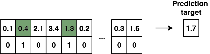
In our rainfall prediction problem, the situation is somewhat less trivial as there is still the additional step of inferring the rainfall ‘numbers’ (the top row) from radar measurements. Furthermore, instead of binary 0/1 values (bottom row) one has continuous time readings between 0 and 60 minutes that have somewhat different roles. Nevertheless, the underlying structural similarities are compelling enough to suggest that RNNs are well-suited for the problem.
In the previous version of this contest (which I did not participate in), gradient boosting was the undisputed star of the show; neural networks, to my knowledge, were not deployed with much success. If RNNs would prove to be as unreasonably effective here as they are in an increasing array of problems in machine learning, then I might have a chance of coming up with a unique and good solution.
For a overview of RNNs, the blog post by Andrej Karpathy is as good a general introduction to the subject as you will find anywhere.
Software and hardware
I used Python with Theano throughout and relied heavily on the Lasagne layer classes to build the RNN architectures. Additionally, I used scikit-learn to implement the cross-validation splits, and pandas and NumPy to process and format the data and submission files. To this day I have an irrational aversion to Matplotlib (even with Seaborn) and so all my plots were done in R.
I trained the models on several NVIDIA GPUs in my lab, which include two Tesla K20 and three M2090 cards.
The data
Pre-processing
From the outset, there were several challenges brought about by certain features of the data:
-
Extreme and unpredictable outliers
-
Variable sequence lengths and irregular radar measurement times
-
A training set with non-independently distributed samples
Extreme and unpredictable outliers
It was well-documented from the start, and much discussed in the competition forum, that a large proportion of the hourly rain gauge measurements were not to be trusted (e.g. clogged rain gauges). Given that some of these values are several orders of magnitude higher than what is physically possible anywhere on earth, the MAE values participants were reporting were dominated by these extreme outliers. However, since the evaluation metric was the MAE rather than the root-mean-square error (RMSE), one can simply view the outliers as an annoying source of extrinsic noise in the evaluation scores; the absolute values of the MAE are however, in my view, close to meaningless without prior knowledge of typical weather patterns in the US midwest.
The approach I and many others took was simply to exclude from the training set the rain gauges with readings above 70mm. Over the course of the competition I experimented with several different thresholds from 53mm to 73mm, and did a few runs where I removed this pre-processing step altogether. Contrary to what was reported in the previous version of this competition, this had very little effect on the performance of the model (positive or negative); it appears, and I speculate, that the RNN models had learnt to ignore the outliers, as suggested by the very reasonable maximum values of expected hourly rain gauge levels predicted for the test set (~45-55mm).
Variable sequence lengths and irregular radar measurement times
The weather radar sequences varied in length from one to 19 readings per hourly rain gauge record. Furthermore these readings were taken at seemingly random points within the hour. In other words, this was not your typical time-series dataset (EEG waveforms, daily stock market prices, etc).
One attractive feature of RNNs is that they accept input sequences of varying lengths due to weight sharing in the hidden layers. Because of this, I did not do any pre-processing beyond removing the outliers (as described above) and replacing any missing radar feature values with zero; I retained each timestamp as a component in the feature vector and preserved the sequential nature of the input. The idea was to implement an end-to-end learning framework and, for this reason, with not a small touch of laziness thrown in, I did not bother to implement any feature engineering.
A training set with non-independently distributed samples
The training set consists of data from the first 20 days of each month and the test set data from the remaining days. This ensures that both sets are more or less independent. However, as was pointed out in the competition forum, because the calendar time and location information is omitted, it is impossible to construct a local validation holdout subset that is truly independent from the rest of the training set; specifically, there is no way of ensuring that any two gauge readings are not correlated in time or space. This had implications in that it was very difficult to detect cases of overfitting without submissions to the public leaderboard (see Training section below for more details).
Data augmentation
One common method to reduce overfitting is to augment the training set via label-preserving transformations on the data. The classic examples in image classification tasks include cropping and shifting the images, and in many cases rotating, perturbing the brightness and colour of the images and introducing noise.
For the radar sequence data, I implemented a form of Dropin augmentation on the data where the sequences were lengthened to a fixed length in the time dimension by duplicating the vectors at random time points. This is loosely speaking the opposite of performing dropout on the input layer, hence the name. This is illustrated in the figure below:
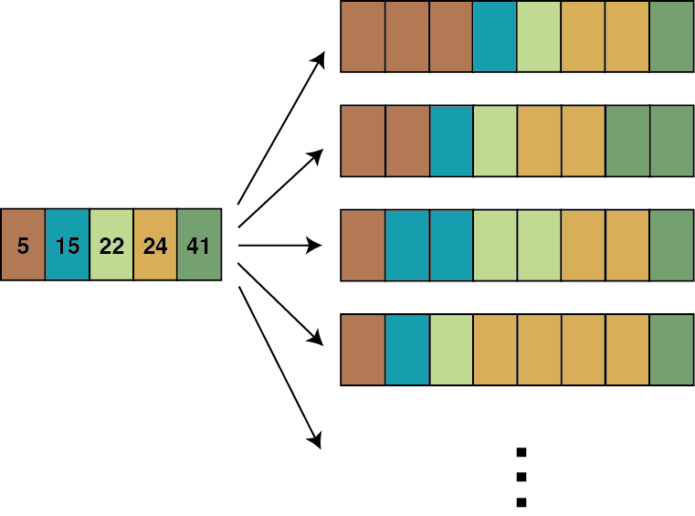
Over the competition I experimented with fixed sequence lengths of 19, 21, 24 and 32 timepoints. I found that stretching out the sequence lengths beyond 21 timesteps was too aggressive as the models began to underfit.
My original intention was to find a way to standardise the sequence lengths to facilitate mini-batch stochastic gradient descent training. However it soon became clear that it could be a useful way to force the network to learn to factor in the time intervals between observations; specifically, this is achieved by encouraging the network to ignore readings when the intervals are zero. To the best of my knowledge this is a novel, albeit simple, idea.
RNN architecture
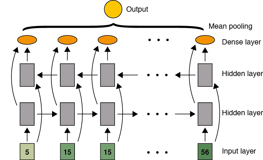
The best performing architecture I found over the competition is a 5-layer deep stacked bidirectional (vanilla) RNN with 64-256 hidden units, with additional single dense layers after each hidden stack. At the top of the network the vector at each time position is fed into a dense layer with a single output and a Rectified Linear Unit (ReLU) non-linearity. The final result is obtained by taking the mean of the predictions from the entire top layer. I will explain the evolution of this model using figures in the following section. This roughly mirrors the way I developed the models over the course of the competition.
Design evolution
The basic model inspired by the adding problem is a single layer RNN:
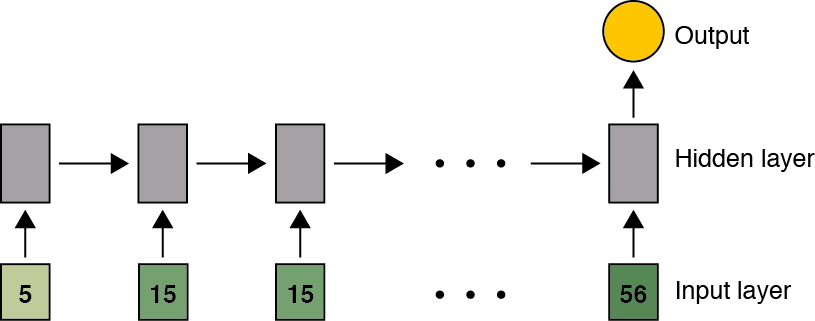
The RNN basically functions as an integration machine and is employed in a many-to-one fashion.
The law of gravity aside, and not to mention the second law of thermodynamics, there is nothing preventing us from viewing the problem as rain flying up from rain gauges on the ground and reconstituting itself as clouds. Hence we can introduce a reverse direction and consider a bidirectional RNN:
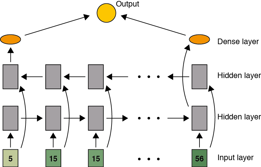
A separate class of architectures imagines predictors situated across the time dimension at the top of the network, each with a unique view to the past and the future. In this scenario we pool together the outputs from the entire hidden layer to obtain a consensus prediction:
Finally, there are all manner of enhancements one can employ to create a deep network such as stacking and inserting dense layers between stacks and at the top of the network (see Pascanu et al.). In addition to these I included a linear layer to reduce the dimension of the feature vectors from 22 to 16, in part to guard against overfitting and partly because the models were beginning to take too long to train (see below):
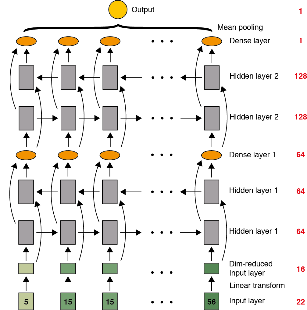
I actually started out with Long-Short Term Memory (LSTM) units but, in order to reduce the training time, switched to ordinary RNNs with fully connected layers, which turned out to be just as effective. My guess is that the advantages of LSTMs are only really apparent for much longer sequences than the radar sequences in this competition.
The final structural idea was to pass the top layer of the network, or perhaps the input layer itself, through a set of 1D convolutional and pooling layers. The motivation for this, other than the irresistable urge to throw the neural network equivalent of the kitchen sink at any and every problem, was the notion of temporal invariance—that the rain collecting in gauges should contribute the same amount to the hourly total regardless of when in the hour it actually entered the rain gauge. In my half-hearted attempt at this, my models unfortunately performed worse and I promptly abandoned it.
Nonlinearities
I used ReLUs throughout with varying amounts of leakiness in the range 0.0-0.5. The goal was not to optimise this hyperparameter but to increase the variance in the final ensemble of models. Nevertheless I did find that using the original ReLU with no leakiness often resulted in very poor convergence behaviours (i.e. no improvement at all).
Training
Local validation
I began by splitting off 20% of the training set into a stratified (with respect to the number of radar observations) validation holdout set. I soon began to distrust my setup as some models were severely overfitting on the public leaderboard despite improving local validation scores. By the end of the competition I was training my models using the entire training set and relying on the very limited number of public test submissions (two per day) to validate the models, which is exactly what one is often discouraged from doing! Due to the nature of the training and test sets in this competition (see above), I believe it was the right thing to do.
Training procedure
I used stochastic gradient descent (SGD) with the Adadelta update rule with a learning rate decay.
I employed mini-batches of size 64 throughout; I found that the models performed consistently worse for sizes of 128 and higher, possibly because the probability of having mini-batches without any of the extreme outliers became very small. I did not get the time to properly investigate this.
Each model was trained over approximately 60 epochs and, depending on the size of the model, the training times ranged from one to five days per model.
Initialisation
Most of the models used the default weight initialisation settings of the Lasagne layer classes. Towards the end of the competition I experimented with the normalized-positive definite weight matrix initialisations proposed in Talathi et al. but found no significant effect on the performances.
Regularisation
My biggest surprise was that implementing dropout resulted in consistently poorer results, contrary to what had been reported by many others, such as in Zaremba et al.. I tried many combinations, including varying the dropout percentage and implementing it only at the top and/or bottom of the network, all without success. This is in stark contrast to the effectiveness of dropout when employed in the fully connected layers of CNN architectures.
For this reason, in the limited time available, I did not bother with weight decay as I reasoned that my main issue was under- rather than overfitting the data.
Model ensembles
Test-time augmentation
To predict each expected rainfall value, I took the mean of 61 separate rain gauge predictions that were generated from different dropin augmentations of the radar data sequence. Implementing this procedure led to a large improvement (~0.03) in the public leaderboard score.
Averaging models
The winning submission was a simple weighted average of 30 separate models. The best model had a public leaderboard score of 23.6971, which should be good enough for fifth place; the worst score in the winning ensemble was 23.7123. The weights were chosen on the basis of a wholly unscientific combination of public leaderboard scores and correlations between the different sets of predictions. Given the difficulties in constructing truly independent splits of the training set, there is no guarantee that the more sophisticated ensembling techniques such as stacked generalisation would be any more effective.
Final thoughts
If I were to take one point away from this contest, it is that the days of manually constructing features from data are almost over. The machines will win. I experienced this in the Plankton classification contest where the monumental effort that my teammate and I put into extracting image features was eclipsed within minutes by even the shallowest of CNNs.
I had lots of fun in this contest and have learnt a lot. Congratulations to the other winners, and special thanks to the competition organisers and sponsors. I will make my code available soon. If you have any questions or comments, please feel free to share them.
UPDATE (2 Jan 2016): The code is now available on GitHub: https://github.com/simaaron/kaggle-Rain